Introduction
如果要判斷某個字的語意,可以用它鄰近的字來判斷,例如以下句子:
The dog run.
A cat run.
A dog sleep.
The cat sleep.
A dog bark.
The cat meows.
The bird fly.
A bird sleep.
由於 dog 和 cat 這兩個字出現在類似的上下文情境中,因此,可以判斷出 dog 和 cat 語意相近。
如果要能夠用數學運算,來計算語意相近程度,可以把文字的語意用向量表示,如下:
其中, dog 的向量為 ( 2, 1, 0, 0, 0, 0, 0, 1, 1, 1 ) ,第一個維度表示 dog 在 a 旁邊的次數有 2 次,第二個維度表示在 bark 旁邊的次數有 1 次,以此類推。
Vector Space of Semantics
有了向量就可以用 cosine similarity 來計算語意相近程度。
給定兩向量 和 ,則這兩向量的 cosine similarity 為:
cosine similarity 算出來的值,即是計算 和 兩向量的夾角的 cosine 值。 cosine 值越接近 1 ,表示兩向量夾角越小,表示兩向量的語意越接近。
根據以上例子, dog ( 2, 1, 0, 0, 0, 0, 0, 1, 1, 1 ) 和 cat ( 1, 0, 0, 0, 0, 0, 1, 1, 1, 2 ) 的 cosine similarity 為:
而 bird 的向量為:( 1, 0, 0, 0, 0, 1, 0, 0, 1, 1 ) ,計算 dog 和 bird 的 cosine similarity :
由於 0.75 > 0.707 ,因此 dog 和 cat 語意比較接近, dog 和 bird 語意比較不同。
此種語意向量有個缺點,就是向量的維度等於總字彙量。例如英文單字種共有好幾萬種,那麼,向量就有好幾萬個維度,向量維度過大的缺點,會造成資料過度稀疏,以及占記憶體的空間。
降低向量維度的方式,有兩種方法,分別是:
-
singular value decompisition (SVD)
-
word2vec
本文先不詳細介紹這部分。
Implementation
在此實作將文字轉成向量,並用 SVD 降為至二維,作視覺化
1
2
3
4
5
6
7
8
9
10
11
12
13
14
15
16
17
18
19
20
21
22
23
24
25
26
27
28
29
30
31
32
33
34
35
36
37
38
39
40
| import numpy as np
import matplotlib.pyplot as plt
text = [
["the", "dog", "run", ],
["a", "cat", "run", ],
["a", "dog", "sleep", ],
["the", "cat", "sleep", ],
["a", "dog", "bark", ],
["the", "cat", "meows", ],
["the", "bird", "fly", ],
["a", "bird", "sleep", ],
]
def build_word_vector(text):
word2id = {w: i for i, w in enumerate(sorted(list(set(reduce(lambda a, b: a + b, text)))))}
id2word = {x[1]: x[0] for x in word2id.items()}
wvectors = np.zeros((len(word2id), len(word2id)))
for sentence in text:
for word1, word2 in zip(sentence[:-1], sentence[1:]):
id1, id2 = word2id[word1], word2id[word2]
wvectors[id1, id2] += 1
wvectors[id2, id1] += 1
return wvectors, word2id, id2word
def cosine_sim(v1, v2):
return np.dot(v1, v2) / (np.sqrt(np.sum(np.power(v1, 2))) * np.sqrt(np.sum(np.power(v1, 2))))
def visualize(wvectors, id2word):
np.random.seed(10)
fig = plt.figure()
U, sigma, Vh = np.linalg.svd(wvectors)
ax = fig.add_subplot(111)
ax.axis([-1, 1, -1, 1])
for i in id2word:
ax.text(U[i, 0], U[i, 1], id2word[i], alpha=0.3, fontsize=20)
plt.show()
|
本程式中, text 是輸入的文字, build_word_vector 將文字轉成向量:
1
| >>> wvectors, word2id, id2word = build_word_vector(text)
|
其中, wvectors 是根據前後文統計後,得出各文字的向量:
1
2
3
4
5
6
7
8
9
10
11
| >>> print wvectors
[[ 0. 0. 1. 1. 2. 0. 0. 0. 0. 0.]
[ 0. 0. 0. 0. 1. 0. 0. 0. 0. 0.]
[ 1. 0. 0. 0. 0. 1. 0. 0. 1. 1.]
[ 1. 0. 0. 0. 0. 0. 1. 1. 1. 2.]
[ 2. 1. 0. 0. 0. 0. 0. 1. 1. 1.]
[ 0. 0. 1. 0. 0. 0. 0. 0. 0. 0.]
[ 0. 0. 0. 1. 0. 0. 0. 0. 0. 0.]
[ 0. 0. 0. 1. 1. 0. 0. 0. 0. 0.]
[ 0. 0. 1. 1. 1. 0. 0. 0. 0. 0.]
[ 0. 0. 1. 2. 1. 0. 0. 0. 0. 0.]]
|
每一橫排(或直排)代表著某個字的向量,但從它看不出是哪個字,所以 word2id 則是給定文字,找出是第幾個向量,而 id2word 則是給定第幾個向量,找出所對應的文字。
1
2
3
4
5
6
7
| >>> print word2id
{'a': 0, 'fly': 5, 'run': 7, 'the': 9, 'dog': 4, 'cat': 3,
'meows': 6, 'sleep': 8, 'bark': 1, 'bird': 2}
>>> print id2word
{0: 'a', 1: 'bark', 2: 'bird', 3: 'cat', 4: 'dog', 5: 'fly',
6: 'meows', 7: 'run', 8: 'sleep', 9: 'the'}
|
例如 dog 是在 wvectors 中, 第 5 排的向量(註:index 從0開始算),用 word2id 可從 wvector 中,取出其對應向量:
1
2
| >>> print wvectors[word2id["dog"]]
[ 2. 1. 0. 0. 0. 0. 0. 1. 1. 1.]
|
程式碼中的 cosine_sim ,則可計算兩向量間的 cosine similarity ,例如,
計算 dog 和 cat 與 dog 和 bird 之間的 cosine similarity :
1
2
3
4
5
| >>> print cosine_sim(wvectors[word2id["dog"]], wvectors[word2id["cat"]])
0.75
>>> print cosine_sim(wvectors[word2id["dog"]], wvectors[word2id["bird"]])
0.707106781187
|
再來是用 visualize 將這些語意向量在平面上作視覺化:
1
| >>> visualize(wvectors, id2word)
|
在平面上作視覺化的方法,是用 SVD 將語意向量降為至二維,就可以把這些向量所對應的字,畫在平面上,結果如下:
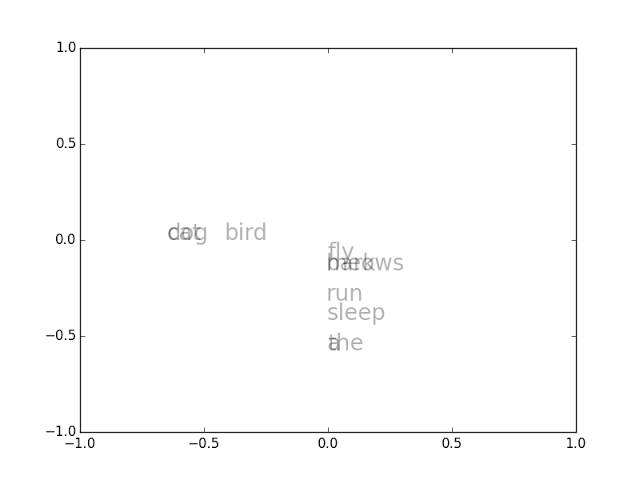
此結果顯示, dog 、 cat 和 bird 是語意相近的一群, a 和 the 語意相近,以此類推。
Further Reading
Simple Word Vector representations
http://cs224d.stanford.edu/lectures/CS224d-Lecture2.pdf