Gradient Descent
機器學習中,用 Gradient Descent 是解最佳化問題,最基本的方法。關於Gradient Descent的公式,請參考:Optimization Method – Gradient Descent & AdaGrad
對於 Cost function ,在 時, Gradient Descent 走的方向為 。也就是,用泰勒展開式展開後,用一次微分 來趨近的方向,如下圖:
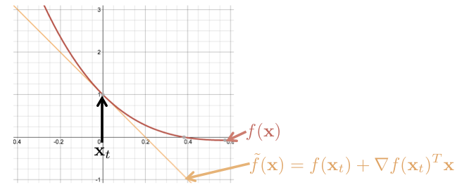
註:考慮到 為向量的情形,故一次微分寫成 。
其中, 為原本的 Cost function ,而 為泰勒展開式取一次微分逼近的。 而 Gradient Descent 走的方向為 ,為沿著 的方向。
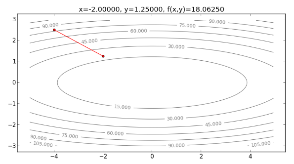
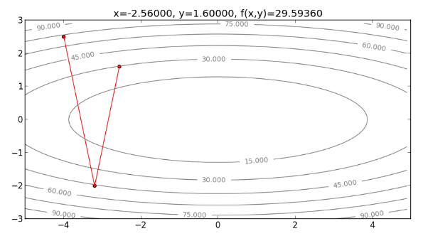
這會有個問題,如果原本的 Cost function 為較高次函數,只用一次項來逼近是不夠的,有時候,失真情形很嚴重,例如, Cost function 為橢圓 , 此函數的等高線圖,如下圖:
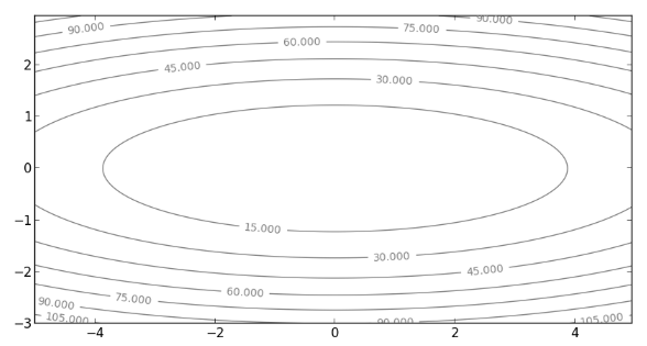
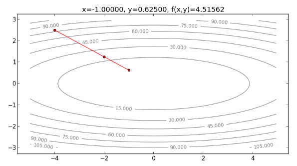
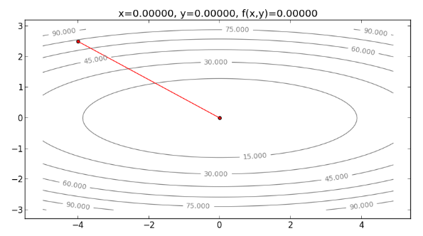
如果起始點為 ,沿著 的方向走,也就是說,走梯度最陡的方向(即與等高線垂直的方向),可能會需要多次折返,才能走到最小值,如下圖:
Second-Order Taylor Approximation
根據前面的例子得知,只考慮一次微分項,是不夠的,現在要來考慮二次微分項。
對於 Cost function , 在 時,用泰勒展開式展開後,分別用一次微分與二次微分來逼近,如下圖:
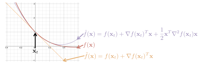
其中,橘色的 為只用了一次微分的逼近,而紫色的 為用了一次與二次微分向的逼近,由此可見, 較 接近原本的
如果要求 的最小值,可以往 為最小值的方向,一步一步走下去。要找出 的最小值,即:
將 對 微分,令微分結果為 ,得:
得
可以用此 ,來當作位於 時,想走往 的最小值,要走的方向(與距離)。用一次與二次微分所得出的方向,一步步走下去,最後走到最小值,這種方法即為 Newton’s Method 。
Newton’s Method for Optimization
Newton’s Method 即是考慮二次微分的 Gradient Descent 方法,公式如下:
其中, 為 Learning Rate , ( 稱為 Hessian ), ( 稱為 Gradient )。
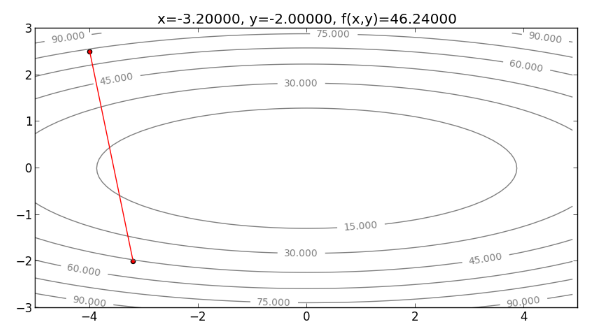
再來看看用 Newton’s Method 來解決 Cost function 為橢圓 的情形。首先,畫出起始點 ,如下圖:

先來算 和 ,分別為:
設 ,代入起始點 、 和 到 Newton’s Method 的公式: ,得:
更新圖上的點, ,如下圖:
再往下走一步,求 的值,如下:
從以上過程發現, Newton’s Method 方向不需要一直折返,可以直接往最小值處走下去 ,整個過程如下圖:

註:事實上,由於本例的 Cost function 為二次函數,如果是用二次的泰勒展開式逼近,則可以完全貼合 。所以用 Newton’s Method 的話, 位於 時, 即是泰勒展開式最小值的 解,也是 的最小值解,如果設 ,只要走一步就可以走到最小值,如下:
過程如下圖所示:
Implementation
再來進入實作的部分
首先,開啟新的檔案 newtons.py 並貼上以下程式碼:
1 2 3 4 5 6 7 8 9 10 11 12 13 14 15 16 17 18 19 20 21 22 23 24 25 26 27 28 29 30 31 32 33 34 35 36 37 38 39 40 41 42 43 44 45 46 47 48 49 50 51 52 53 54 55 56 57 58 59 60 61 62 63 64 65 66 67 | |
其中, obj_func(x,y) 為目標函數, obj_func_grad(x,y) 為 , obj_func_hessian(x,y) ,而 plot_function(xt,yt,c='r') 可畫出目標函數的等高線圖, run_gd() 用來執行 Gradient Descent , run_newtons() 用來執行 Newton’s Method 。 xy 對應到前例的 ,而 eta 為 Learning Rate 。 for i in range(20) 表示最多會跑20個迴圈。
到 python console 執行:
1
| |
執行 Gradient Descent ,指令如下:
1
| |
則程式會逐一畫出整個過程:
以此類推
執行 Newton’s Method ,指令如下:
1
| |
則程式會逐一畫出整個過程:

以此類推
Comment
Newton’s Method 需要計算二次微分 Hessian 矩陣的反矩陣,如果 variable 為高維度向量,則計算這個矩陣的時間複雜度會很高,而且很占記憶體空間,因此有人提出一些 Hessian 矩陣的近似求法,例如 L-BFGS 。但如果用在像是 Deep Learning 這種有超多 variable 的模型,近似求法仍然太慢,因此解 Deep Learning 問題,通常只會用一次微分的方法,例如 Adagrad之類的。
Reference
本文參考至以下教科書:
Stephen Boyd & Lieven Vandenberghe. Convex Optimization. Chapter 5 Duality.