1.Motivation
本文接續先前提到的 Overfitting and Regularization
Machine Learning – Overfitting and Regularization
探討如何避免 Overfitting 並選出正確的 Model
因為 Overfitting 的緣故, 所以無法用 來選擇要用哪個 Model
在上一篇文章中, 可以把 最小的 Model 當成是最佳的 Model , 但是在現實生活的應用中, 無法這樣選擇, 因為, 在訓練 Model 時,無法事先知道 Testing Data 的預測結果是什麼 ,所以就不可能用 來選擇 Model
既然這樣, 要怎麼辦呢? 既然不可以用 來選擇 Model , 又無法事先算出
2.Validation Set
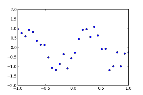
例如, 用高次多項式做 Linear Regression , 假設只有一群 Training Data , 如下圖藍色點, 沒有 Testing Data , 要怎麼辦呢?
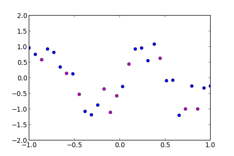
有個解決方法, 就是在 Training Data 中, 隨機選取某一部份 當作 Testing Data , 在訓練過程中不去使用, 這些 Data 稱為 Validation Set ,如下圖紫色的點
用圖中藍色的點, 訓練出一個 Model , 如下圖
訓練完之後, 再用 Validation Set 算 Error , 這個 Error 稱作 Validation Error , ,可用於挑選最佳的 Model
至於 Validation Set 要挑多少 Data ? , 挑太多會導致 Training Data 的量大減少太多, 而無法訓練出準確的 Model , 但挑太少則會使得 Validation Error 被少數的點給 Bias , 所以, 通常是選取 Training Data 的 ~ 左右的量, 作為 Validation Set
3.Implementation of Validation Set
接著來實作, 先來看看 Training Data 要怎麼切割
開新的檔案 mdselect.py 並貼上以下程式碼
mdselect.py 1
2
3
4
5
6
7
8
9
10
11
12
13
14
15
16
17
18
19
20
21
22
23
24
25
26
27
28
29
30
31
32
33
34
35
36
37
38
import numpy as np
import matplotlib.pyplot as plt
from operator import itemgetter
data_tr = [
( 0.9310 , - 0.3209 ), ( - 0.3103 , - 1.1853 ), ( - 0.7241 , 0.8071 ), ( 0.6552 , - 1.1979 ), ( - 1.0000 , 0.9587 ),
( - 0.5172 , 0.1218 ), ( 0.3793 , 1.0747 ), ( - 0.7931 , 0.9202 ), ( 0.1724 , 0.9259 ), ( - 0.2414 , - 0.8748 ),
( 0.5862 , - 0.0751 ), ( 0.2414 , 0.9573 ), ( 1.0000 , - 0.2715 ), ( - 0.6552 , 0.3408 ), ( - 0.3793 , - 1.0831 ),
( 0.0345 , - 0.2877 ), ( 0.5172 , - 0.0876 ), ( 0.3103 , 0.5422 ), ( - 0.9310 , 0.7560 ), ( 0.7931 , - 0.2613 ),
( 0.8621 , - 1.0038 ), ( - 0.1724 , - 0.3660 ), ( - 0.0345 , - 0.5762 ), ( 0.1034 , 0.4364 ), ( - 0.8621 , 0.5780 ),
( - 0.5862 , 0.1347 ), ( - 0.1034 , - 1.1036 ), ( 0.7241 , - 1.0032 ), ( - 0.4483 , - 0.5247 ), ( 0.4483 , 0.6258 ),
]
data_ts = [
( 0.1034 , 0.4559 ), ( 0.5172 , 0.6431 ), ( - 0.1724 , - 1.1199 ), ( 0.7931 , - 0.9601 ), ( 0.7241 , - 1.4629 ),
( - 0.6552 , 1.1571 ), ( - 0.0345 , - 0.3840 ), ( 0.2414 , 0.9064 ), ( 0.5862 , - 0.2830 ), ( - 1.0000 , 0.8299 ),
( 0.1724 , 1.1434 ), ( 0.3103 , 0.7773 ), ( - 0.3103 , - 1.3973 ), ( - 0.9310 , 0.5383 ), ( - 0.4483 , - 0.6886 ),
( - 0.5172 , - 0.2233 ), ( - 0.2414 , - 0.7119 ), ( - 0.1034 , - 0.3853 ), ( - 0.7241 , 0.9869 ), ( - 0.7931 , 0.9888 ),
( 0.6552 , - 0.8112 ), ( - 0.8621 , 0.9862 ), ( - 0.3793 , - 1.0019 ), ( 0.3793 , 0.6254 ), ( 0.0345 , - 0.1150 ),
( 1.0000 , - 0.0712 ), ( 0.8621 , - 0.8452 ), ( 0.4483 , 0.0301 ), ( - 0.5862 , - 0.4771 ), ( 0.9310 , - 0.7827 ),
]
def data_split ( s1 , s2 ):
return data_tr [: s1 ] + data_tr [ s2 :] , data_tr [ s1 : s2 ]
def plot_data ( d_tr = None , d_val = None , d_ts = None , d_m = None , title = '' ):
plt . ion ()
fig , ax = plt . subplots ()
for d , c in [( d_tr , 'bo' ),( d_val , 'mo' ),( d_ts , 'ro' )]:
if d != None :
ax . plot ( map ( itemgetter ( 0 ), d ), map ( itemgetter ( 1 ), d ), c )
if d_m != None :
ax . plot ( np . array ( map ( itemgetter ( 0 ), d_m )), np . array ( map ( itemgetter ( 1 ), d_m )), 'k--' )
ax . set_xlim (( - 1 , 1 ))
ax . set_ylim (( - 2 , 2 ))
ax . set_title ( title )
plt . show ()
其中 , data_tr 和 data_t 分別是 Training Data 和 Testing Data , 這些 Data 都已經先隨機洗牌過,因此用 Index 的順序抽出的 Data 都已經是隨機的, 不會依序剛好抽到一筆連續的 Data , 而 data_split 是用來切割 Data 用的 function , plot_data 是畫圖用的
到 python 的 interactive mode 載入模組
1
>>> import mdselect as ms
用 data_split(s1,s2) 就可以把 Training Data 分開, 例如我想要把第 1~10 筆資料抽出來, 作為 Validation Set , 方法如下
1
2
3
4
5
6
7
8
9
10
11
12
>>> dtr , dval = ms . data_split ( 0 , 10 )
>>> dtr
[( 0.5862 , - 0.0751 ), ( 0.2414 , 0.9573 ), ( 1.0 , - 0.2715 ), ( - 0.6552 , 0.3408 ), \
( - 0.3793 , - 1.0831 ), ( 0.0345 , - 0.2877 ), ( 0.5172 , - 0.0876 ), ( 0.3103 , 0.5422 ), \
( - 0.931 , 0.756 ), ( 0.7931 , - 0.2613 ), ( 0.8621 , - 1.0038 ), ( - 0.1724 , - 0.366 ), \
( - 0.0345 , - 0.5762 ), ( 0.1034 , 0.4364 ), ( - 0.8621 , 0.578 ), ( - 0.5862 , 0.1347 ), \
( - 0.1034 , - 1.1036 ), ( 0.7241 , - 1.0032 ), ( - 0.4483 , - 0.5247 ), ( 0.4483 , 0.6258 )]
>>> dval
[( 0.931 , - 0.3209 ), ( - 0.3103 , - 1.1853 ), ( - 0.7241 , 0.8071 ), ( 0.6552 , - 1.1979 ), \
( - 1.0 , 0.9587 ), ( - 0.5172 , 0.1218 ), ( 0.3793 , 1.0747 ), ( - 0.7931 , 0.9202 ), \
( 0.1724 , 0.9259 ), ( - 0.2414 , - 0.8748 )]
其中 dtr 是 Training Data , dval 是 Validation Set
再來, 用 plot_data 把資料畫出來
1
>>> ms . plot_data ( d_tr = dtr , d_val = dval )
再來, 就是用 Training Data 來訓練 Model , 用 Validation Set 計算 Validation Error
到 mdselect.py 貼上以下程式碼
mdselect.py 1
2
3
4
5
6
7
8
9
10
11
12
13
14
15
16
17
18
19
20
21
22
23
24
25
26
def model_train ( order , split = None , plot = True , show_eout = False ):
if split != None :
d_tr , d_val = data_split ( split [ 0 ], split [ 1 ])
d_ary = [ d_tr , d_val , data_ts ]
else :
d_ary = [ data_tr , data_ts ]
X_ary = map ( lambda d : np . matrix ( map ( lambda x :
map ( pow , [ x ] * ( order + 1 ), range ( order + 1 )), map ( itemgetter ( 0 ), d )))
, d_ary )
Y_ary = map ( lambda d : np . matrix ( map ( itemgetter ( 1 ), d )) , d_ary )
w = np . linalg . pinv ( X_ary [ 0 ] ) * Y_ary [ 0 ] . T
y_ary = map ( lambda X : ( X * w ) . T , X_ary )
E_ary = map ( lambda Y , y : np . average ( np . square ( Y - y )) , Y_ary , y_ary )
p_model = sorted ( reduce ( add , map ( lambda i : zip ( map ( itemgetter ( 0 ), d_ary [ i ]),
map ( lambda j : y_ary [ i ][ 0 , j ], range ( y_ary [ i ] . shape [ 1 ])))
, range ( len ( d_ary ) - 1 ))), key = itemgetter ( 0 ))
if plot != False :
if split != None : d_val = d_ary [ 1 ]
else : d_val = None
if show_eout == True : d_out = d_ary [ - 1 ]
else : d_out = None
plot_data ( d_ary [ 0 ], d_val , d_out , p_model , "order= %s " % ( order ))
return E_ary
第一個參數是 order 是多項式的次數, 第二個參數是 split 就是要切出來做 Validation Set 的 Data , 預設為 split=None 表示把所有的 Training Data 都當成 Training Data , 剩下的參數, plot 選擇是否要畫圖, show_eout 選擇是否要在圖上顯示
修改完 mdselect.py 要重新載入
1
2
>>> reload ( ms )
< module 'mdselect' from 'mdselect.py' >
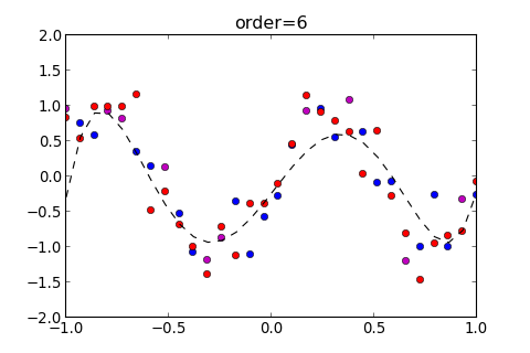
如果是用六次多項式來訓練, 而 Validation Set 是第 1~10 筆資料, 用法如下
1
2
>>> ms . model_train ( order = 6 , split = ( 0 , 10 ))
[ 0.085523976119494666 , 0.34656284169000939 , 0.16791141763767087 ]
這個 function 會回傳三個參數, 依序為 , 並會自動畫出以下圖形
如果要在圖上顯示 , 則設定參數 show_eout=True , 如下
1
2
>>> ms . model_train ( order = 6 , split = ( 0 , 10 ), show_eout = True )
[ 0.085523976119494666 , 0.34656284169000939 , 0.16791141763767087 ]
接著, 要找出 最小的 Model 是哪一個, 需要依序用不同的 Order 來訓練不同的 Model
再到 mdselect.py 貼上以下程式碼
mdselect.py 1
2
3
4
5
6
7
8
9
10
11
12
13
14
15
16
17
18
19
20
21
22
23
24
25
26
27
28
29
30
31
32
33
def model_select ( split = None , o1 = 3 , o2 = 11 ):
result = map ( lambda o : ( o , model_train ( o , split , plot = False )), range ( o1 , o2 ))
rmin = min ( result , key = lambda x : x [ 1 ][ 1 ])
for order , err in result :
if split != None :
print "Order: %s , Ein: %.5f , Eval: %.5f , Eout: %.5f " % ( order , err [ 0 ], err [ 1 ], err [ 2 ])
else :
print "Order: %s , Ein: %.5f , Eout: %.5f " % ( order , err [ 0 ], err [ 1 ])
print "Min Result:"
if split != None :
print "Order: %s , Ein: %.5f , Eval: %.5f , Eout: %.5f " % ( rmin [ 0 ], rmin [ 1 ][ 0 ], rmin [ 1 ][ 1 ], rmin [ 1 ][ 2 ])
else :
print "Order: %s , Ein: %.5f , Eout: %.5f " % ( rmin [ 0 ], rmin [ 1 ][ 0 ], rmin [ 1 ][ 1 ])
plot_model_select ( result , split , o1 , o2 )
def plot_model_select ( result , split , o1 , o2 ):
x = [ order for order , _ in result ]
d = [ err for _ , err in result ]
fig , ax = plt . subplots ()
if split != None :
tp_ary = [( 0 , 'bo' , 'b--' , 'Ein' ),( 1 , 'mo' , 'm--' , 'Eval' ),( 2 , 'ro' , 'r--' , 'Eout' )]
else :
tp_ary = [( 0 , 'bo' , 'b--' , 'Ein' ),( 1 , 'ro' , 'r--' , 'Eout' )]
for tp in tp_ary :
ax . plot ( x , map ( itemgetter ( tp [ 0 ]), d ) , tp [ 2 ], label = tp [ 3 ])
ax . plot ( x , map ( itemgetter ( tp [ 0 ]), d ) , tp [ 1 ])
ax . set_xlim (( o1 , o2 ))
ax . set_ylim (( 0 , 1 ))
ax . set_xlabel ( 'Order' )
ax . set_ylabel ( 'Error' )
plt . legend ()
plt . show ()
修改完 mdselect.py 重新載入
1
2
>>> reload ( ms )
< module 'mdselect' from 'mdselect.py' >
這個 function 會依序從 訓練到 , 並把 的值畫成圖表, 以及找出 最小的 Order 是哪一個
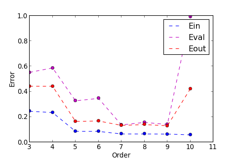
例如用第 1~10 筆為 Validation Set ,選出最佳的 Model ,如下
1
2
3
4
5
6
7
8
9
10
11
>>> ms . model_select ( split = ( 0 , 10 ))
Order : 3 , Ein : 0.24487 , Eval : 0.55254 , Eout : 0.44307
Order : 4 , Ein : 0.23451 , Eval : 0.58775 , Eout : 0.44250
Order : 5 , Ein : 0.08565 , Eval : 0.32730 , Eout : 0.16432
Order : 6 , Ein : 0.08552 , Eval : 0.34656 , Eout : 0.16791
Order : 7 , Ein : 0.06510 , Eval : 0.13649 , Eout : 0.13285
Order : 8 , Ein : 0.06497 , Eval : 0.15669 , Eout : 0.13948
Order : 9 , Ein : 0.06431 , Eval : 0.14018 , Eout : 0.13009
Order : 10 , Ein : 0.05805 , Eval : 0.99262 , Eout : 0.42279
Min Result :
Order : 7 , Ein : 0.06510 , Eval : 0.13649 , Eout : 0.13285
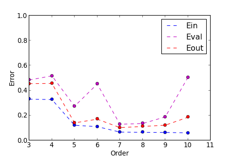
結果顯示, 在 時 , 有最小的 , 也為最小, 程式畫出圖表如下
圖中有三條線, 其中紫色的線為 , 這條線的趨勢和紅色的線 類似, 所以可以用來選擇最佳的 Model
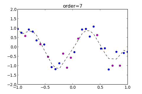
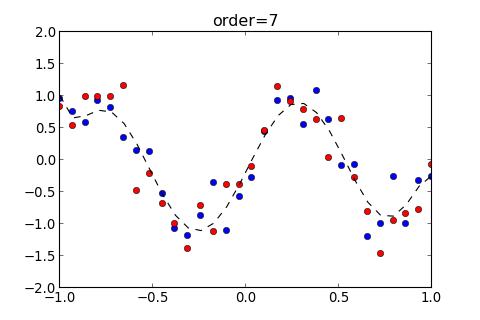
可以把 的 Model 也畫出來看看, 如下
1
2
>>> ms . model_train ( 7 , split = ( 0 , 10 ), show_eout = True )
[ 0.065103000120556462 , 0.13648767336843776 , 0.13284787573861817 ]
4.Train Again !
由於選出 Validation Set 會使得原本的 Training Data 變少, 但是用更多的 Training Data 來訓練, 是有可能使 降得更低
所以, 在選好 Model 以後, 可以把 Validation Set 也併入 Training Data , 再訓練一次, 這樣就有可能把 降低
用 model_train 訓練剛才得出的最佳 Order , 也就是 , 但這次用參數 split=None , 就是不要切割出 Validation Set
1
2
>>> ms . model_train ( 7 , split = None , show_eout = True )
[ 0.071946203316513205 , 0.096047913185552308 ]
得出以上結果, 可知, 用所有的 Training Data 做訓練, 結果為 比起剛剛, 有切出 Validation Set 的 下降一些
所以經由 Validation Set 找出了參數 Order 以後, 再用全部的 Training Data 都訓練過一次, 的確可以把 降低
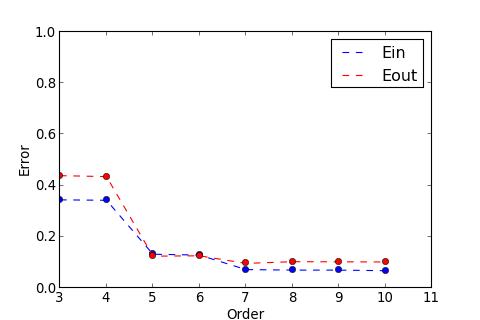
來看看用全部的 Training Data 訓練來挑 Order 參數, 誰的 最小,用 model_select 參數輸入 split=None , 結果如下
1
2
3
4
5
6
7
8
9
10
11
>>> ms . model_select ( split = None )
Order : 3 , Ein : 0.34432 , Eout : 0.43882
Order : 4 , Ein : 0.34271 , Eout : 0.43519
Order : 5 , Ein : 0.13194 , Eout : 0.12439
Order : 6 , Ein : 0.12855 , Eout : 0.12578
Order : 7 , Ein : 0.07195 , Eout : 0.09605
Order : 8 , Ein : 0.06991 , Eout : 0.10288
Order : 9 , Ein : 0.06987 , Eout : 0.10224
Order : 10 , Ein : 0.06754 , Eout : 0.10167
Min Result :
Order : 7 , Ein : 0.07195 , Eout : 0.09605
這次運氣很好, 用 Validation Set 就成功挑出了 最小的 Order 參數, 但事實上, 未必每次運氣都這麼好
5.V-fold Cross Validation
運氣不好的時候, 選的 Validation Set , 和 的分佈型態有所差距, 以至於用 無法找出 最小的Model
1
2
3
4
5
6
7
8
9
10
11
>>> ms . model_select ( split = ( 15 , 25 ))
Order : 3 , Ein : 0.45906 , Eval : 0.13305 , Eout : 0.45137
Order : 4 , Ein : 0.45786 , Eval : 0.12820 , Eout : 0.44651
Order : 5 , Ein : 0.10279 , Eval : 0.31029 , Eout : 0.12523
Order : 6 , Ein : 0.09748 , Eval : 0.30769 , Eout : 0.12489
Order : 7 , Ein : 0.03825 , Eval : 0.17898 , Eout : 0.09523
Order : 8 , Ein : 0.02848 , Eval : 0.22228 , Eout : 0.11895
Order : 9 , Ein : 0.02838 , Eval : 0.23299 , Eout : 0.12376
Order : 10 , Ein : 0.02832 , Eval : 0.25718 , Eout : 0.12957
Min Result :
Order : 4 , Ein : 0.45786 , Eval : 0.12820 , Eout : 0.44651
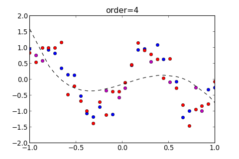
由上圖紫色的線看到, 的趨勢和 很不一樣, 把 的 Model 畫出來, 看看出了什麼問題
1
2
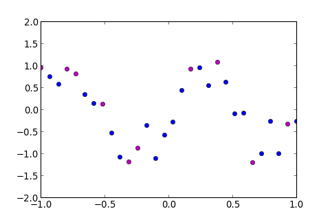
>>> ms . model_train ( 4 , split = ( 15 , 25 ), show_eout = True )
[ 0.45785961181234375 , 0.12819567955706512 , 0.44650895269797458 ]
從下圖可知, 我們運氣真的很不好, 因為挑到的點的 y 值都在中間, 所以會選出這樣的 Model
那這種情況要怎麼避免呢?
有種方法叫作 V-fold Cross Validation , 就是把 Training Data 切成 份, 總共訓練 次, 每次訓練從 份中挑一份作為 Validation Set , 剩下的 份當作 Training set , 最後再把每一次計算所得出的 Error 平均起來, 詳細過程如下
把 Training Data 切成 , 先挑一份作為 Validation Set
得出 Validation Error :
再挑一份不同的 Data 為 Validation Set , 如下
得出 Validation Error :
這樣重複進行 次, 直到每一份 都當過 Validation Set , 再把所有算出來的 Validation Error 平均起來
這樣可避免 Validation Error 受到運氣不好的 Validation Set 的影響, 而選出不好的 Model
Implementation of V-fold CV
再到 mdselect.py 貼上以下程式碼
mdselect.py 1
2
3
4
5
6
7
8
9
10
11
12
13
14
15
16
17
18
19
20
21
22
23
24
25
26
27
def v_fold ( o1 = 3 , o2 = 11 ):
result = map ( lambda o : ( o , np . average ( np . matrix (
map ( lambda s : model_train ( o , split = ( s * 6 ,( s + 1 ) * 6 ), plot = False ), range ( 5 )))
, axis = 0 )), range ( o1 , o2 ))
rmin = min ( result , key = lambda x : x [ 1 ][ 0 , 1 ])
for order , err in result :
print "Order: %s , Ein: %.5f , Eval: %.5f , Eout: %.5f " % ( order , err [ 0 , 0 ], err [ 0 , 1 ], err [ 0 , 2 ])
print "Min Result:"
print "Order: %s , Ein: %.5f , Eval: %.5f , Eout: %.5f " % ( rmin [ 0 ], rmin [ 1 ][ 0 , 0 ], rmin [ 1 ][ 0 , 1 ], rmin [ 1 ][ 0 , 2 ])
plot_vfold ( result , o1 , o2 )
def plot_vfold ( result , o1 , o2 ):
x = [ order for order , _ in result ]
y_ary = map ( lambda i : [ err [ 0 , i ] for _ , err in result ] , [ 0 , 1 , 2 ])
tp_ary = [( 0 , 'bo' , 'b--' , 'Ein' ),( 1 , 'mo' , 'm--' , 'Eval' ),( 2 , 'ro' , 'r--' , 'Eout' )]
fig , ax = plt . subplots ()
for tp in tp_ary :
ax . plot ( x , y_ary [ tp [ 0 ]] , tp [ 2 ], label = tp [ 3 ])
ax . plot ( x , y_ary [ tp [ 0 ]] , tp [ 1 ])
ax . set_xlim (( o1 , o2 ))
ax . set_ylim (( 0 , 1 ))
ax . set_xlabel ( 'Order' )
ax . set_ylabel ( 'Error' )
plt . legend ()
plt . show ()
其中 v_fold 就是 V-fold Cross Validation 演算法 , 在這 function 中, 也就是把 Training Data 切成五份 , 並把其中一份挑出來做 Validation Set
修改完 mdselect.py 重新載入
1
2
>>> reload ( ms )
< module 'mdselect' from 'mdselect.py' >
執行 v_fold ,結果如下
1
2
3
4
5
6
7
8
9
10
11
>>> ms . v_fold ()
Order : 3 , Ein : 0.33048 , Eval : 0.48405 , Eout : 0.45466
Order : 4 , Ein : 0.32709 , Eval : 0.51738 , Eout : 0.45618
Order : 5 , Ein : 0.12095 , Eval : 0.27391 , Eout : 0.14044
Order : 6 , Ein : 0.11037 , Eval : 0.45183 , Eout : 0.17004
Order : 7 , Ein : 0.06660 , Eval : 0.12957 , Eout : 0.10250
Order : 8 , Ein : 0.06446 , Eval : 0.13500 , Eout : 0.11171
Order : 9 , Ein : 0.06402 , Eval : 0.18829 , Eout : 0.12179
Order : 10 , Ein : 0.06035 , Eval : 0.50482 , Eout : 0.18569
Min Result :
Order : 7 , Ein : 0.06660 , Eval : 0.12957 , Eout : 0.10250
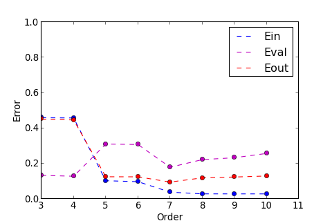
v_fold 找出了 時, 有最小的 , 也有最小的
以上圖表顯示 , 紫色的線和紅色的線, 趨勢也不會差太遠, 也可用於選擇 最小的 Model
事實上, V-fold Cross Validation 未必每次都能找出 最小的 Model , 因為它是由各種不同的結果所平均起來的, 也會受到較差結果者的影響, 但至少比較不會因為 運氣不好 而挑到不好的 Validation Set
6.Reference
本文參考至以下兩門 Coursera 線上課程
1.Andrew Ng. Machine Learning
https://www.coursera.org/course/ml
2.林軒田 機器學習基石 (Machine Learning Foundations)
https://www.coursera.org/course/ntumlone