1.Introduction
這次來講一下機器學習(Machine Learning)
簡而言之,Machine Learning是一種讓機器根據已知的data,預測出未知的data情形如何
現在,來看看一種簡單的Machine Learning演算法
叫作Perceotron Algorithm
Peceptron Algorithm要做的事
就是要讓電腦學習,怎樣畫一條線,把兩群不同的資料分開
2.Load Data
接著來看看要怎麼實作Perceptron Algorithm
首先,開啟新的檔案 perceptron.py 並載入模組
1 2 | |
給定一筆資料
1 2 3 4 5 6 7 8 9 10 11 12 13 14 15 16 17 | |
其中 X1 是資料的X座標, X2 是資料的Y座標, Y是資料的分類的結果, 不是Y座標
然後寫個function 把data畫出來
1 2 3 4 5 6 7 8 9 | |
到interactive mode執行
1 2 | |

這個圖把藍色( ),和紅色( )兩群資料呈現出來
3.Draw Line
再來,看看怎麼畫一條線
先在 perceptron.py 檔案新增一個畫線的function
我們要畫的這條線有兩個參數,分別是
這條線的直線方程式是:
藉由改變 的數值,我們可以控制這條線的斜率
*註:
事實上若只有只可以改變線的斜率,必須再另外再加個常數相才可改變線的位置
本文提到的是較簡化的模型,故省略常數項*
1 2 3 4 5 6 7 8 9 10 11 12 13 14 15 16 17 18 19 20 21 22 23 24 25 26 27 | |
程式碼有點多,但其實是為了處理某些special case,例如 ` w2 != 0 :` 是用來判斷斜率是否為無限大
到interactive mode載入模組
1 2 | |
接著你可以試著輸入不同的參數,讓電腦畫出不同的線,例如:
1 2 3 4 | |


這樣就可以畫出不一樣的線了
改變數字大小,可控制斜率
改變正負號,可以把紅色或藍色的區域反轉過來
4. Perceptron Algorithm
接下來,我們要讓電腦自己去學習,該怎麼樣畫一條線把資料分開
Peceptron Algorithm 的概念是這樣
先隨便給一條線,然後再根據這條線分類錯誤做修正
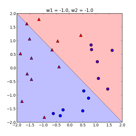
我們先給定畫出一條線,如下圖
從上圖中分類錯誤的點中,任意挑一個點 ,
用 到原點的向量 ,來修正直線的法向量
要怎麼修正呢?要看 的類別 來決定, 調整 的方向
公式如下:
用這個方法就可以改變直線的斜率,把分類錯誤的點 ,歸到正確的一類,
舉例:
1.藍色( )分類錯誤
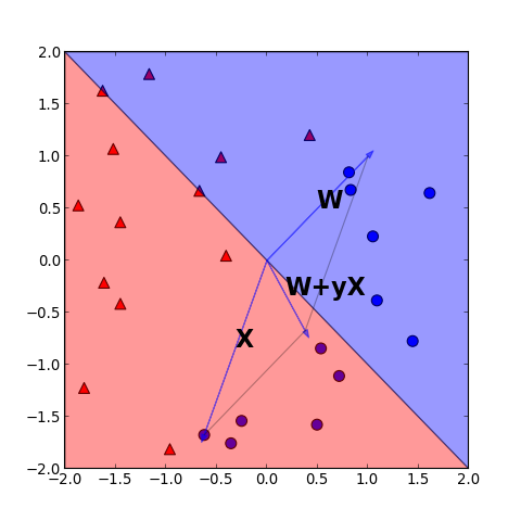
修正後如下

2.紅色( )分類錯誤

修正後如下
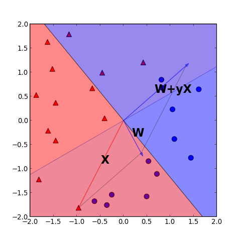
以上結果顯示, 修正過後, 有可能會把原本分類正確的點,分類到錯的一類
所以可能要重複修正好幾次,直到把所有的點都分類正確為止
所以Perceptron的演算法如下:
(1) 任選一條線
(2) 從這條線中選一個分類錯誤的點x
(3) 由點x修正線的斜率
(4) 重複(2)直到所有的點都分類正確
我們把這個演算法寫到 perceptron.py 裡
1 2 3 4 5 6 7 8 9 10 11 | |
寫好之後,到interactive mode載入模組後,
其中times是迴圈的最大重複次數,
如果超過這個次數後還沒有完全分類正確,則演算法停止
1 2 3 4 5 6 7 8 9 10 | |
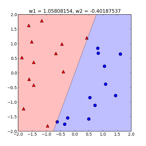
總共執行了五次迴圈,所有的分類就都正確了
執行結果如下:
如果想要看看每一次迴圈中修正 的情形
以下提供更詳盡過程分解
但程式碼有點長
1 2 3 4 5 6 7 8 9 10 11 12 13 14 15 16 17 18 19 20 21 22 23 24 25 26 27 28 29 30 31 32 33 34 35 36 37 38 39 40 41 42 43 44 45 46 47 48 49 50 51 52 53 54 55 56 57 58 59 60 61 62 63 64 65 66 67 68 69 70 71 72 73 74 75 76 | |
然後,到interactive mode跑看看這個function
1 2 3 4 5 6 7 | |
進行完每次計算時,程式會把圖畫出來
然後程式會暫停,要按下ENTER才能繼續進行下一步
執行結果如下:

5. Further Reading
以上是Perceptron Algorithm很簡單的介紹
但其實Perceptron Algorithm有其他變化形式
例如,如果有noise存在的時候,本篇介紹的演算法就無法求得最佳解
就要用其他的變化形式來處理
想要看更多相關介紹,請到coursera上線上課程
1.Andrew Ng. Machine Learning
https://www.coursera.org/course/ml
2.林軒田 機器學習基石 (Machine Learning Foundations)
https://www.coursera.org/course/ntumlone